Introduction

During the initial testing phase of our developed Web application, there arose a need for Web server benchmarking. Since the performance results of the system to be deployed kept on fluctuating while loading / publish the concerned data, this also followed when there was an increase in number of user accessing the system. Explaining the conditions of these fluctuating performances to the client was a nightmare. So we were in a desperate need to estimate the web server performance in order to find the characteristics of the server during high workload. The solution we came across was to use JMeter, which is an Apache based load testing tool.

Apache JMeter

Apache JMeter is a pure Java application designed to measure the performance of application servers and database servers used to host web applications (load test client /server software). It may be used to test performance both on static and dynamic resources such as static files, Java Servlets, ASP.NET, PHP, CGI scripts, Java objects, databases, FTP servers, and more. JMeter can be used to simulate a heavy load on a server, network or object to test its strength or to analyze overall performance under different load types. Additionally, JMeter can help in regression testing of application and to validate that application.

Parameters of the application testing

The key parameters that generally needs to be measured regarding the performance for a web server application are,

• Number of requests that can be served per second.

• Latency response time in milliseconds for each new connection or request

• Throughput in bytes per second (depending on file size, cached or not cached content, available network bandwidth, etc.).

• The measurements must be performed under a varying load of clients and requests per client.

All these conditions were taken into account in designing / customizing the tool to the project needs, like setting time to send requests & to wait for the responses.

JMeter Setup

Before the actual setup of JMeter, the system should have Java installed in it. Because JMeter is pure Java desktop application, it requires a fully compliant JVM 6 or higher. You can download and install the latest version of Java SE Development Kit, which is available in the above link http://www.oracle.com/technetwork/java/javase/downloads/index.html.

1. After installation is finished, you can use the following procedure to check whether Java JDK is installed successfully in your system

   • In Window/Linux, go to command prompt / Terminal

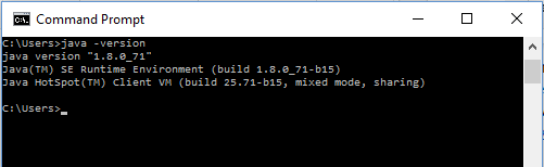
     Enter command “java -version”
     If Java runtime environment is installed successfully, you will see the output as the figure below

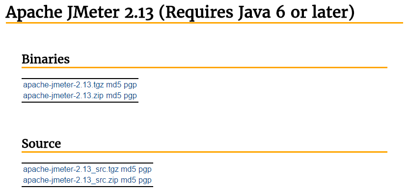
2. Download JMeter, the latest version of Apache JMeter can be downloaded from the site http://jmeter.apache.org/download_jmeter.cgi. Download any of the compressed zip/tar file from the Binaries section.

3. Installation of JMeter is extremely easy and simple. You simply unzip the zip/tar file into the directory where you want JMeter to be installed, preferably in C:/ drive. There is no tedious installation screen to deal with, Simple unzip and you are done.

4. Given below is the description of the JMeter directories and its importance JMeter directory contains many files and directory

   • /bin: Contains JMeter script file for starting JMeter

   • /docs: JMeter documentation files

   • /extras: ant related extra files

   • /lib/: Contains the required Java library for JMeter

   • /lib/ext: contains the core jar files for JMeter and the protocols

   • /lib/junit: JUnit library used for JMeter

5. Launching JMeter can be done in 3 modes

   • GUI Mode

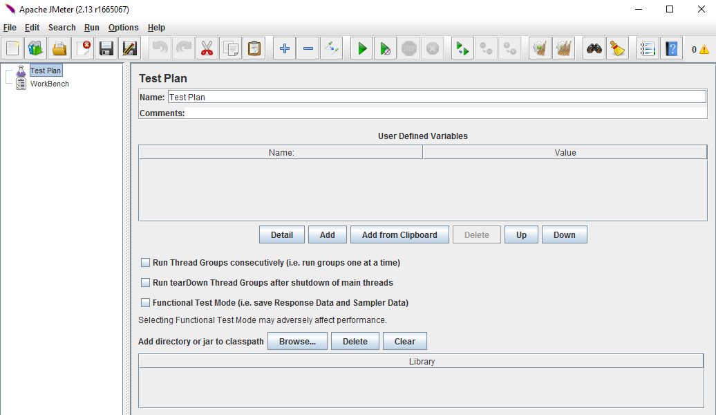
If you are using Window, just run the file jmeter.bat from the directory  C:\apache-jmeter-2.13\bin which here is the installed directory to start JMeter in GUI mode.

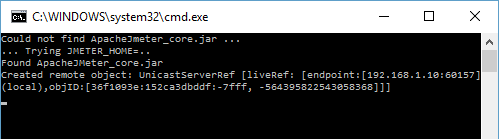
• Server Mode

Server mode is used for distributed testing. This testing works as client-server model. In this model, JMeter runs on server computer in server mode. On client computer, JMeter runs in GUI mode. To start the server mode, you run the file jmeter-server.bat from the same directory path.

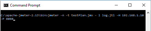
• Command Line Mode

JMeter in GUI mode consumes much computer memory. For saving resource, you may choose to run JMeter without the GUI. This is a command line for example jmeter -n -t testPlan.jmx – l log.jtl -H 192.168.1.1 -P 8080 (will not work on other system, since port and host has to be modified) Where,

jmeter–n: Shows that JMeter will run on command line mode

-t testPlan.jmx: Name of file contains the Test plan

– llog.jtl: Shows the log files which contains the test result

-H 192.168.1.1 -P 8080: Proxy server host name and port

Setting up a test plan using JMeter

Test plan is set to run performance tests in order to evaluate the performances of the server when serving WMS requests. The performance test aim to stress the server and evaluate the response time with an increasing number of simulated users sending concurrent request to the server.

1. Since we do the testing from client side, we prefer the JMeter GUI. Start JMeter and add a new Thread Group with a right click over Test Plan option in the test plan pane.

2. A new thread group is created on which Right click and then add Loop Controller from Logic Controllers. After which in the thread group panel, set the number of thread for the test (this represents the number of simultaneous requests that are made to GeoServer) and the ramp-up period. Also, check Forever on the Loop Count field.

For example, if you enter a Ramp-Up Period of 5 seconds, JMeter will finish starting all of your users by the end of the 5 seconds. So, if we have 5 users and a 5 second Ramp-Up Period, then the delay between starting users would be 1 second (5 users / 5 seconds = 1 user per second). If you set the value to 0, then JMeter will immediately start all of your users.

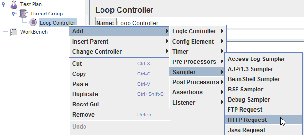
3. Right click on the Loop Controller and add a new HTTP Request element from Sampler option.

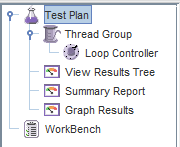
4. Add the following listeners by right clicking on Test Plan: View results Tree, Summary Report, Graph results.

5. In the HTTP Request enter the basic configurations of host address, port number and the path.

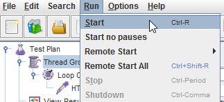
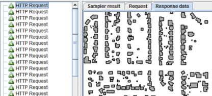
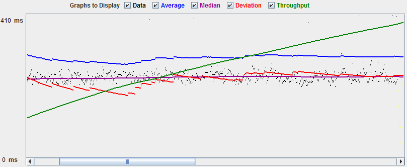
6. After this step the JMeter is configured to run a GeoServer performance test, Now click Run option and Start the test. After the test is done / stop, Select View Results Tree to directly see the request informations produced and the request result, Select Summary report to view the statistical information about the requests and Select Graph Results to analyze the trend of the requests.

The above setup is just the basic configuration to run JMeter, so based on this the requests were modified to hold and test the Web map server data of our AOI and the performance report was generated.

Discussion on the measured performance

After the application was set up in the server, we checked the performance characteristics of a few locations from our project Area of Interest. These area are referred in the article as Region A and Region B. These two regions were chosen in random, but had marked contrast in the features present and the density of it as well. The testing was designed in a way that the AOI will be rendered at the Zoomed out state initially (Level 0) and working towards greater detailing zoomed in state (Level 9). At each level the performance characteristics were computed based on the load (No. of users accessing). Also this test was performed through both Internet and Intranet, to obtain the performance of the server without the influence of external factors such as internet bandwidth.

Before we go into the performance details, let us talk about the 2 areas which were chosen. Region B was a complete built up area with dense buildings and roads and a lot of heterogenous features, whereas Region A was a mixture of a small portion of built up area surrounded by a huge mass of sandy soil, basically a lot more homogenous. When the results of the performance were obtained, like the difference in land cover of the area, the characteristic graph was also different. Generally we would obtain 3 sets of performance data for each region, which being Minimum time, Maximum time and Average time. Average time provides the actual picture on the system performance, since Minimum and Maximum time depends on a lot of other varying factors which might throw the analysis of track. Hence Average time performance were alone considered.

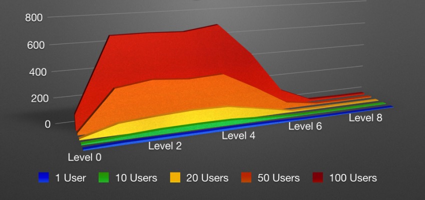
Region A

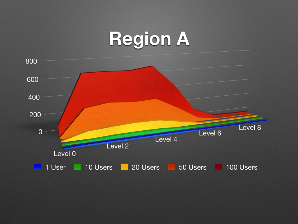
The above figure provides the performance characteristic of our developed system based on different load conditions while loading Region A. Level 0 is predictable of it being quick to load, since the resolution of the loaded tiles is lesser. When the region is zoomed the resolution of each pixel increases and thus there seems to be an increase in the average loading time of the data, which gets exaggerated when the load on the increases. But at certain level this condition did not hold true and the loading time decreased, which at first seemed strange because greater the resolution greater the amount of distinguishable heterogenous features and thus greater the time taken to load each tile in the system. Since this region had very minimal built up area and maximum coverage of homogenous sandy terrain, the average loading time went down.

Region B

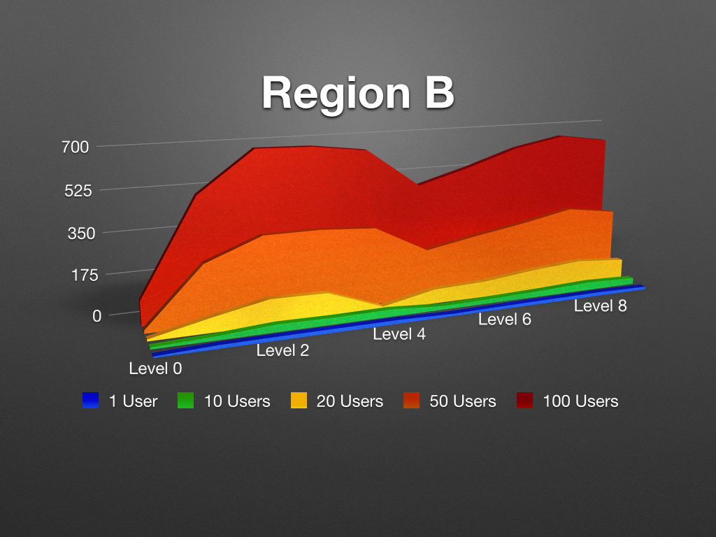
Similar to region A, this above figure provides the performance characteristic of our developed system based on different load conditions while loading Region B. Here from Level ) till Level 5 the characteristics remain more or less similar to that of Region A. But that is where the similarities end, since from Level 5 it again starts to rise and reach a plateau till level 9. This change in characteristic is attributed to the fact that the area being loaded is heterogenous and thus there is time to load increases. There is dip at Level 5 (middle) because there is a marked difference in the amount of tiles being loaded in the canvas, even though the resolution is increasing. This is the same reason the system performance reaches a plateau from Level 6 to 9, since the tiles being rendered remains the same.

From these performance characteristic graph our web server performance was arrived which was latter shared with the client on request, this also considerably reduced the time we spent explaining the client on fluctuations in rendering time of the system. Also helped us in identifying the places that the application needed fixing to obtain better performance.